
Image generated by O3
TL;DR: We’re going to “fine-tune” a 7B-parameter Mistral model over there in Google Colab!
Recently I had a very different idea: I wanted an LLM model to play Minecraft by itself, that way I wouldn’t need to mine diamonds, but I don’t think Steve would like that proposal very much⛏️
From that point on, I started thinking about a strategy to create a model and how I could make it read Minecraft commands. Luckily for me, there is Minecraft Malmo, which allows the game data to be exposed, making it easier to read the environment, leaving only the LLM part. I also found out that they even already made a scientific paper about a similar idea.
Initially I thought about doing a Fine Tunning on the first GPT 2 model from Open AI. Thinking about using commands in Portuguese, I switched to one of the GPT 2 models already in Portuguese with 114M parameters. Even though it worked, it didn’t seem to be enough. We needed more firepower. So I thought about a few possibilities, between a 7B-parameter Mistral model and the 13B-parameter LLAMA model. In some benchmarks, the Mistral model outperforms the Llama model and it is a small model, ideal for running a test. The training was done in Google Colab, you can follow it in practice by accessing the full notebook here.
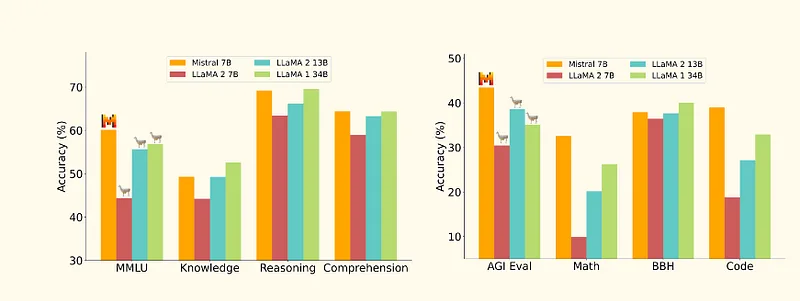
https://mistral.ai/news/announcing-mistral-7b
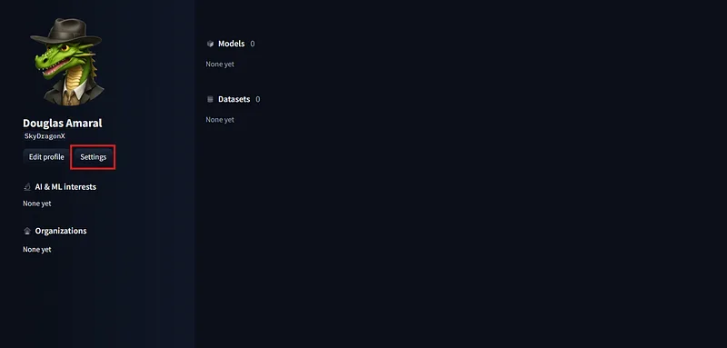
Before starting the code part, you will need to do two things. The first one, still outside Google Colab, is to create a HuggingFace account and generate an access token. After creating your account, go to your profile and click on settings (Settings)
You will see a side menu with your user-specific settings, click on AccessTokens and then on Create New Token. Set your Token with Read permission
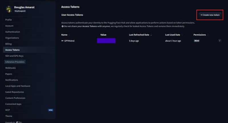
After completing the step above, you will see a screen with your Token. Copy your Token key and there in Google Colab, add it to your notebook’s “Secrets”. Look for the icon that looks like a key, it should be listed as Secrets. Add your token with the key name HF_TOKEN. It is important to add it as HF_TOKEN, otherwise you won’t be able to import the model “on the fly” from HuggingFace.
After completing these steps, you can start development in blocks in Google Colab. Here you have two alternatives:
- Write the code in several blocks, which I recommend, because that way if some part of the code breaks, you can fix it and run it again
- Writing the code in a single block is simpler, but if training breaks, you will have to run everything from scratch.
The first part of the code is the libraries that you should import so your model works correctly. You can create a block just for the imports.
!pip install -q -U transformers accelerate bitsandbytes
!pip install -q -U peft trl datasets
To give you an idea of what each library does, here is a short description of each one.
**transformers**– 🚂
Hugging Face’s parent library; it brings the models (GPT-like, BERTs, Mistral, etc.), tokenizers, and generation APIs. It is where you load, use, and save the model after your fine tune, that is, your fine tuning.**accelerate**– ⚡
Abstracts hardware details (CPU, GPU, multi-GPU, TPU) and distributes training without headaches. You write once, it “accelerates” on any infra.**bitsandbytes**– 🪙
Implements very lightweight 8-bit / 4-bit quantization and optimizations to reduce VRAM and memory usage. Essential for QLoRA or cheap inference.**peft**– 🎛️
Parameter-Efficient Fine-Tuning: Lets you train only a fraction of the parameters (adapters), saving time and GPU. One example is LoRA, which we’re going to use here.**trl**– 🎮
Transformers Reinforcement Learning. Makes RLHF(Reinforcement Learning from Human Feedback), DPO, and similar things on top of 🤗 models easier. Useful if you want to tune with human feedback or preference optimization.**datasets**– 📚
Does download, streaming, preprocessing, and splitting of datasets in a fast format (Arrow). Integrates natively withtransformersand accepts JSONL, CSV, Parquet, almost anything.
Now that you have already created the first block in Google Colab with the imports, we can move on to our second code block.
import os
from google.colab import drive

# Mount your your GDrive on Google Colabs
drive.mount('/content/drive',  force_remount=True)

# Your Path on Google Drive - You must change it
BASE_FOLDER = "/content/drive/MyDrive/Colab Notebooks/GPTMinecraft/"
# -----------------------------------------

# Define the Path of Files
TRAIN_FILE = os.path.join(BASE_FOLDER, "train.txt")
OUTPUT_DIR = os.path.join(BASE_FOLDER, "mistral-7b-minecraft-agent")

assert os.path.exists(TRAIN_FILE), f"Trainer file not found: {TRAIN_FILE}"
We are setting up your Drive folder in Google Colabs. You will need to grant Drive access permission and also define where the folder will be. I recommend keeping force_remount as True to avoid access issues in case you have to Restart the Session.
And of course, you need to define the name of your training file and what the output of your tuned model will be. In my case, my file has several pieces of data like this here:
{"text":"[TAREFA] criar bancada_de_trabalho [INVENTÁRIO] {\"tronco_de_carvalho\":6} [AÇÃO] craft tabuas"}Training File
The idea is that when my character receives some information from Malmo, it decides to take an action based on what it already has in the inventory. So for that I created 3 special tokens. [TASK][INVENTORY][ACTION]
- [TASK] The action that should be performed, depending on the information it receives from the world.
- [INVENTORY] Which items it currently has in the inventory
- [ACTION] What it should do based on its Task and Inventory.
It works, but it only started giving decent results after around one thousand examples. The biggest challenge is making the model learn craft logic — after all, it is only trying to predict the next token.
- Fixed markers (inside brackets) avoid ambiguity for the tokenizer.
- Snake_case or kebab-case for item names keeps everything in few tokens, saving context. I would personally prefer to use camelCase, but who created the training file was Gemini, so it stayed at its discretion. And an important point: with snake_case we use fewer tokens!
- Valid JSON makes parsing the training data easier if later you want structured extraction.
- Always close each entry with
</s>(or your tokenizer’s EOS token) so context does not “leak” between examples. - If the dataset grows, consider a
.jsonlwith a"text"field that contains exactly this full string. And you can always structure your training with JSON, XML, that’s the magic of LLMs - In English models tend to have a much larger vocabulary, so depending on what you want to do, it might be better to train in English.
In the middle of creating the tutorial, I changed the training file from a TXT to a JSONL.
Tokenizer
The tokenizer is perhaps the most important part if you want to Fine Tune a model. It is responsible for splitting and transforming the text sent to the LLM into tokens.
We move on to our third code block:
import torch
import transformers
import os
from transformers import AutoModelForCausalLM,
AutoTokenizer, BitsAndBytesConfig


model_id = "mistralai/Mistral-7B-Instruct-v0.3"

tokenizer = AutoTokenizer.from_pretrained(model_id, use_fast=True,
trust_remote_code=True)

special = {"additional_special_tokens": [
    "[TAREFA]", "[INVENTÁRIO]", "[AÇÃO]",
    "[ITEM]", "[QUANTIDADE]", "[MATERIAL]",
    "[FERRAMENTA]", "[CRAFT]", "[COLETAR]"
]}
tokenizer.add_special_tokens(special)
tokenizer.pad_token = tokenizer.eos_token
tokenizer.padding_side = "right"

# --- now load quantized model with matching vocab size ----
bnb_cfg = BitsAndBytesConfig(load_in_4bit=True, bnb_4bit_quant_type="nf4",
                             bnb_4bit_compute_dtype=torch.bfloat16,
                             bnb_4bit_use_double_quant=True)

model = AutoModelForCausalLM.from_pretrained(
    model_id,
    quantization_config=bnb_cfg,
    device_map="auto",
    trust_remote_code=True,
)
model.resize_token_embeddings(len(tokenizer))

# quick sanity batch
batch = tokenizer(
    ["[TAREFA] criar bancada_de_trabalho [INVENTÁRIO] {\"tronco\":3} [AÇÃO]",
     "[TAREFA] fazer espada_de_ferro [ITEM] espada [MATERIAL] ferro"],
    return_tensors="pt",
    padding=True,
    add_special_tokens=True
).to(model.device)

with torch.no_grad():
    _ = model(**batch)
print("✅ Model & tokenizer Ready!")
Perfect, let’s split this block into parts so you understand what we are doing in each little part of it.
tokenizer = AutoTokenizer.from_pretrained(model_id, use_fast=True,
trust_remote_code=True)
We are passing to our tokenizer the model Id that we are going to use, whether it will have fast mode (which uses a tokenizer made in Rust, not all models can use it), and whether we trust the repository to use the model’s custom Tokens. This option is only advisable if the model is trustworthy. If you want to know more about AutoTokenizer and the possible parameters, just access the official documentation over on HuggingFace
special = {"additional_special_tokens": [
    "[TAREFA]", "[INVENTÁRIO]", "[AÇÃO]",
    "[ITEM]", "[QUANTIDADE]", "[MATERIAL]",
    "[FERRAMENTA]", "[CRAFT]", "[COLETAR]"
]}
tokenizer.add_special_tokens(special)
tokenizer.pad_token = tokenizer.eos_token
tokenizer.padding_side = "right"
In this block above, we are adding a few extra tokens to the model, so it can distinguish when it receives a command and the next action. As for pad_token=eos_token, we are telling the model that if there is an empty space on the right, it should fill it with the same ending token, in our case </s>. This ends up being a pattern used in Fine Tunnings of LLMs.
bnb_cfg = BitsAndBytesConfig(load_in_4bit=True, bnb_4bit_quant_type="nf4",
                             bnb_4bit_compute_dtype=torch.bfloat16,
                             bnb_4bit_use_double_quant=True)
Here we are using something called quantization. Instead of storing each number with a high-precision float (for example, using 32 bits, known as float32), quantization stores them with much lower precision (in this case, 4 bits). This results in drastic memory savings, allowing models that would normally require 40GB of VRAM to fit on GPUs with much less. On HuggingFace you can check more details on how each quantization stage works, or even check the official documentation, also on HF.
model = AutoModelForCausalLM.from_pretrained(
    model_id,
    quantization_config=bnb_cfg,
    device_map="auto",
    trust_remote_code=True,
)
model.resize_token_embeddings(len(tokenizer))

# quick sanity batch
batch = tokenizer(
    ["[TAREFA] criar bancada_de_trabalho [INVENTÁRIO] {\"tronco\":3} [AÇÃO]",
     "[TAREFA] fazer espada_de_ferro [ITEM] espada [MATERIAL] ferro"],
    return_tensors="pt",
    padding=True,
    add_special_tokens=True
).to(model.device)

with torch.no_grad():
    _ = model(**batch)
print("✅ Model & tokenizer Ready!")
Now that we have all the configurations, let’s load the model and do one final check.
- Loading the Model: We use
AutoModelForCausalLM.from_pretrainedto load our model. The key point here is to pass our quantization configuration (quantization_config=bnb_cfg), which will apply 4-bit compression in real time. We also usedevice_map="auto"so that Hugging Face automatically manages the allocation of the model on the GPU. - Adjusting the Embeddings: Next, we call
model.resize_token_embeddings. This step is crucial to synchronize the model with the tokenizer, especially if we added new special tokens, ensuring that there will be no dimension errors. If when training your model you did not add anything, you do not need to worry about this. - Sanity Check: Before starting the training loop, we create a small example batch (
batch), tokenize it, and pass it through the model. This is done inside awith torch.no_grad()block to save memory, since we are only testing the data flow (inference), not training. If this step completes without errors, we receive the confirmation message and can be sure that our data pipeline is working perfectly, ready for fine-tuning! Now we will move on to LoRA, which may deserve a slightly larger section.
LoRA (Low Rank Adaptation)
from peft import LoraConfig, get_peft_model

# LoRA Config
# Defines what part of the model will be trained
lora_config = LoraConfig(
    r=16,
    lora_alpha=32,
    target_modules=[
        "q_proj", "k_proj", "v_proj", "o_proj",
        "gate_proj", "up_proj", "down_proj"
    ],
    lora_dropout=0.05,
    bias="none",
    task_type="CAUSAL_LM"
)

model = get_peft_model(model, lora_config)
print("🔧 Lora Config Applied:")
model.print_trainable_parameters()
The concept of LoRA is somewhat important in LLM scenarios. Instead of training all the billions of parameters of the original model (which would be computationally very expensive and require a lot of VRAM), we freeze the entire model and inject small “adaptable layers” (in strategic places. Only these new layers, which are tiny by comparison, will be trained. If you have been working with LLMs for a while, you should know that there are also more LoRAs for Stable Difussion, where we inject specific layers for images. That way, you can have an anime style, Pixel ART, more realistic or not, using image models directly on your computer in the style of LM Studio. If you got curious, you can look at some image models and LoRAs on Civit.Ai.
In the case of our LLM, let’s understand what this code means step by step.
lora_config = LoraConfig(
    r=16,
    lora_alpha=32,
    target_modules=[ "q_proj", "k_proj", "v_proj", "o_proj",
    "gate_proj", "up_proj", "down_proj"],
    lora_dropout=0.05,
    bias="none",
    task_type="CAUSAL_LM"
)**r=16**(Rank): This is the most important parameter in LoRA. It defines the “size” or the “capacity” of our adapter layers. Technically, it is the rank of the low-rank matrix we are using to approximate the weight update. Think ofras a dimensional “bottleneck”. A largerrcreates adapters with more parameters, allowing them to learn more complex tasks, but at the cost of more VRAM and training time. A smallerris more efficient, but may not have the capacity to learn nuances. Common values are 8, 16, 32, or 64.**lora_alpha=32**: This is a scaling parameter for LoRA adapters. The output of the adapters is multiplied by a factor oflora_alpha / r. Think oflora_alphaas the “volume” of the adapters’ learning. By defininglora_alphaas doubler(a common practice), we are giving more weight to the information learned by the LoRA adapters. This helps prevent the new information from being “muffled” by the magnitude of the original frozen model weights.**target_modules=[...]**: Here we specify exactly where in the model we are going to inject our LoRA adapters. Why these modules? The names"q_proj","k_proj","v_proj","o_proj","gate_proj", etc., correspond to the linear layers inside the attention blocks and feed-forward networks of the Transformer. These are the most critical layers for the model’s learning and adaptation. By targeting them, we get the maximum “bang for the buck” (best result for the lowest cost). The exact list can vary a bit depending on the model architecture (Llama, Mistral, etc.).**lora_dropout=0.05**: Applies a dropout layer only on the LoRA adapters. It is a standard regularization technique that helps prevent overfitting on the new weights that are being trained, randomly zeroing 5% of activations during training. That way, the “specialists” in your LLM model take a break at each training step, encouraging the model not to depend excessively on any individual neuron in the LoRA layer.**bias="none"**: Specifies which bias parameters will be trained. The"none"option is the most efficient and common, indicating that we will not train any bias, only the weights of the LoRA matrices. The fewer parameters we use for training the better, less VRAM and faster.**task_type="CAUSAL_LM"**: Informs the PEFT library that we are working with a Causal Language Model. This helps the library configure the architecture correctly for the next-word prediction task. Other models are SEQ_2_SEQ_LM, SEQ_CLS, TOKEN_CLS… We are not going to go deeper into them, but they are more for labeling training, features, sentiment analysis, and so on.
model = get_peft_model(model, lora_config)
print("🔧 Lora Config Applied:")
model.print_trainable_parameters()
In this part here, we are loading our previous model and injecting the LoRA settings. This way, we “freeze” the other parameters and define only the parameters we are going to retrain, which we defined above. And to ensure that we got the LoRA configuration right, we print these parameters. With everything correct, we can move on to the next steps.
Model training
import json
import os
import torch
from datasets import load_dataset
from transformers import TrainingArguments, TrainerCallback
from trl import SFTTrainer, SFTConfig

class ValidationCallbackV03(TrainerCallback):
    def __init__(self, tokenizer):
        self.tokenizer = tokenizer
        self.best_base_rate = 0
        self.valid_count= 0

    def on_evaluate(self, args, state, control, model, **kwargs):
        if state.global_step > args.warmup_steps and state.global_step % 75 == 0:
            self.valid_count += 1
            print(f"\n🧪 Validation v0.3 #{self.valid_count} - Step {state.global_step}")
            print("=" * 60)

            base_rate = self.validate_model(model)

            if self.valid_count > 2:
                if base_rate < 45 and self.best_base_rate > 70:
                    print("🛑 Regression Detected! Stopping...")
                    control.should_stop = True
                elif base_rate < 25:
                    print("🛑 Critical Regression Detected! Stopping...")
                    control.should_stop = True

            self.best_base_rate = max(self.best_base_rate, base_rate)

    def validate_model (self, model):
        CRITICAL_TESTS = [
            # Basic Tests
            ("criar picareta_de_madeira", {"tabuas_de_carvalho": 3,
"graveto": 2}, "craft picareta_de_madeira", "basic"),
            ("criar cama", {"tabuas_de_carvalho": 3, "la": 3},
"craft cama", "basic"),
            ("criar espada_de_ferro", {"barra_de_ferro": 2,
"graveto": 1}, "craft espada_de_ferro", "basic"),
            ("obter barras_de_ferro", {"minerio_de_ferro_cru": 5,
"carvao": 2, "fornalha": 1}, "fundir minerio_de_ferro_cru", "basic"),
            ("criar bancada_de_trabalho", {"tronco_de_carvalho": 3},
"craft tabuas", "basic"),

            # Reasoning Tests
            ("criar picareta_de_ferro", {"graveto": 2},
"obter barras_de_ferro", "reasoning"),
            ("criar espada_de_diamante", {"graveto": 1},
"coletar diamante", "reasoning"),
            ("criar fornalha", {"pedregulho": 7},
"coletar pedregulho", "reasoning"),
        ]

        basic_fails = 0
        total_basic = 0
        reasoning_fails = 0
        total_reasoning = 0


        for task, inventory, expected, category in CRITICAL_TESTS:
            inventory_str = str(inventory).replace("'", '"')
            prompt = f"[TAREFA] {task} [INVENTÁRIO] {inventory_str} [AÇÃO]"

            inputs = self.tokenizer(prompt, return_tensors="pt",
add_special_tokens=False)
            inputs = {k: v.to(model.device) for k, v in inputs.items()}

            with torch.no_grad():
                outputs = model.generate(
                    **inputs,
                    max_new_tokens=25,
                    do_sample=False,
                    pad_token_id=self.tokenizer.eos_token_id,
                    eos_token_id=self.tokenizer.eos_token_id,
                    repetition_penalty=1.05
                )

            new_tokens = outputs[0][inputs['input_ids'].shape[1]:]
            response = self.tokenizer.decode(new_tokens,
skip_special_tokens=True)
            response = response.split('<|endoftext|>')[0].strip()

            right = expected in response
            status = "✅" if right else "❌"

            print(f"{status} {category.upper()}: {task}")
            print(f"   Expected: {expected}")
            print(f"   Response: {response}")

            if category == "basic":
                total_basic += 1
                if not right:
                    basic_fails += 1
            else:
                total_reasoning += 1
                if not right:
                    reasoning_fails += 1

        base_basic_rate = (total_basic - basic_fails) / total_basic * 100
        base_reason_rate = (total_reasoning - reasoning_fails) / total_reasoning * 100 if total_reasoning > 0 else 0.0


        print(f"\n📊 RESULTS v0.3:")
        print(f"   Basic Hit Rate:
{base_basic_rate:.1f}% ({total_basic - basic_fails}/{total_basic})")
        print(f"   Reasoning Hit Rate:
{base_reason_rate:.1f}% ({total_reasoning - reasoning_fails}/{total_reasoning})")
        print(f"   Best History Rate: {self.best_base_rate:.1f}%")

        return base_basic_rate

# ===== DATASET CONFIG =====
print("📂 Loading dataset...")


raw_ds = load_dataset("json", data_files={"train": TRAIN_FILE})["train"]

# ➋ Split 85 / 15
ds_split = raw_ds.train_test_split(test_size=0.15, seed=42)

print(f"📊 Dataset split:")
for split, ds in ds_split.items():
    print(f"   {split.capitalize():10s}: {len(ds):,} examples")


tok_kwargs = dict(
    add_special_tokens=True,
    truncation=True,
    max_length=512,
    padding="max_length"
)

def tokenize(batch):
    return tokenizer(batch["text"], **tok_kwargs)

tokenized = ds_split.map(
    tokenize,
    batched=True,
    remove_columns=["text"]
)

training_args = SFTConfig(
    output_dir=OUTPUT_DIR,
    per_device_train_batch_size=2,
    gradient_accumulation_steps=6,
    learning_rate=8e-5,
    bf16=True,
    tf32=True,
    num_train_epochs=15,
    save_steps=50,
    eval_steps=50,
    logging_steps=15,
    save_strategy="steps",
    eval_strategy="steps",
    warmup_steps=125,
    load_best_model_at_end=True,
    metric_for_best_model="eval_loss",
    greater_is_better=False,
    save_total_limit=4,
    warmup_ratio=0.18,
    lr_scheduler_type="cosine",
    report_to="none",
    dataloader_pin_memory=False,
    remove_unused_columns=False,
    prediction_loss_only=True,
    packing=False,
    max_seq_length=512,
    dataloader_num_workers=4,
    group_by_length=True,
    weight_decay=0.02,
    max_grad_norm=0.5

)

# ===== TRAINER CONFIG =====
print("🔧 Config Trainer to v0.3...")

validation_callback = ValidationCallbackV03(tokenizer)
trainer = SFTTrainer(
    model=model,
    train_dataset=tokenized["train"],
    eval_dataset=tokenized["test"],
    peft_config=lora_config,
    args=training_args,
    processing_class = tokenizer,
    callbacks=[validation_callback]

)

# ===== TRAINING=====
print("🚀 Starting Training...")
print(f"📊 Dataset: {len(tokenized['train'])}
training examples, {len(tokenized['test'])} validation examples")
print(f"⚙️ Config: {training_args.num_train_epochs}
epochs, LR={training_args.learning_rate}")
print("=" * 70)


# Train
trainer.train()

# ===== Saving Model =====
print("\n💾 Saving model..")

# Save PreTrained Model
trainer.model.save_pretrained(OUTPUT_DIR)
tokenizer.save_pretrained(OUTPUT_DIR)

# Save Config Model
config = {
    "base_model": model_id,
    "task_type": "minecraft_agent",
    "special_tokens": special,
    "max_seq_length": 512,
    "learning_rate": training_args.learning_rate,
    "num_epochs": training_args.num_train_epochs,
    "batch_size": training_args.per_device_train_batch_size,
    "gradient_accumulation": training_args.gradient_accumulation_steps
}

with open(os.path.join(OUTPUT_DIR, "training_config.json"), "w") as f:
    json.dump(config, f, indent=2)

print(f"✅ Complete Model Saved On: {OUTPUT_DIR}")
print(f"📋 Config Saved On: {OUTPUT_DIR}/training_config.json")

print("\n🧪 Final Validation v0.3...")
final_rate = validation_callback.validate_model(trainer.model)
print(f"🎯 Final Hit Rate: {final_rate:.1f}%")

print("🎉 Mistral Training v0.3 completed!")

def compare_tokenizer():

    test_examples = [
        "[TAREFA] criar picareta_de_madeira
[INVENTÁRIO] {\"tabuas_de_carvalho\": 3, \"graveto\": 2} [AÇÃO] craft picareta_de_madeira",
        "[TAREFA] fazer bancada_de_trabalho
[INVENTÁRIO] {\"tronco_de_carvalho\": 5} [AÇÃO] craft tabuas",
        "[TAREFA] obter barras_de_ferro
[INVENTÁRIO] {\"minerio_de_ferro_cru\": 5, \"carvao\": 2, \"fornalha\": 1}
[AÇÃO] fundir minerio_de_ferro_cru"
    ]

    print("\n🔍 Token Analisis v0.3:")
    print("=" * 50)

    for i, example in enumerate(test_examples, 1):
        tokens = tokenizer.encode(example)
        decoded = tokenizer.decode(tokens)

        print(f"Examples {i}:")
        print(f"  Text: {example[:60]}...")
        print(f"  Tokens: {len(tokens)}")
        print(f"  Eficiency: {len(example) / len(tokens):.2f} chars/token")
        print(f"  Reconstruction: {'✅' if decoded.strip() == example.strip()
 else '❌'}")
        print()

compare_tokenizer()
Finally, we are getting close to the final part of our training, the moment when we will actually train the model. By the way, if you looked at the code, you must have noticed that we are doing validation by steps and not by epochs, which is usually the most common. When training large language models, the point of ‘best performance’ can be reached very quickly, sometimes even before completing a single pass through the dataset (an epoch). By evaluating every 50 steps, we get fast and granular feedback on progress. This allows us to:
- Identify problems early: If loss is not decreasing, we will know in minutes, not hours.
- Capture the best model: With
load_best_model_at_end=True, theTrainercan identify the best checkpoint with high precision (for example, at step 850), something an epoch-based strategy (which would save at step 1000) would miss. - Enable effective Early Stopping: Our
ValidationCallbackcan detect regression and stop training at the right moment, saving resources.
For a Fine Tuning, the step-based training approach may be better than the epoch-based one, but it all depends on what you intend to do, the number of steps, epochs… I’m not an expert on what the best choice should be, but you can check the official Trainer documentation to choose the best path.
And to make sure our model does not just improve its loss score, but also learns the tasks we care about, we create a custom ValidationCallback.
This class works as an ‘inspector’ that, every 75 steps, pauses training and submits the model to a series of practical tests that we define. More importantly, it implements early stopping logic: if the model starts making mistakes on basic tasks it had already mastered, training is interrupted. This protects us against “catastrophic forgetting” and ensures that we save the best version of our model. I’m not going to go into detail on the whole process, but basically we are validating all inputs.
raw_ds = load_dataset("json", data_files={"train": TRAIN_FILE})["train"]
ds_split = raw_ds.train_test_split(test_size=0.15, seed=42)
In this part of loading the dataset, we are loading the JSON and splitting it into 85% for training and 15% for validation. We use the seed to ensure that the random data split is always the same every time the code is run. The number 42 is just to make sure we find the Answer to the Universe.
tok_kwargs = dict(
    add_special_tokens=True,
    truncation=True,
    max_length=512,
    padding="max_length"
)
Here, we are simply creating a dictionary to group the settings that we will use to tokenize the text. This keeps the code cleaner.
**add_special_tokens=True**: Instructs the tokenizer to add the model’s special tokens, such as<s>(start of sequence) and</s>(end of sequence), to each text example.**truncation=True**: If a text example is longer thanmax_length, it will be cut off (truncated) to avoid errors.**max_length=512**: Defines the maximum length of each sequence. This number generally depends on the model’s capacity or the GPU memory limitations.**padding="max_length"**: If a text example is shorter thanmax_length, padding tokens ([PAD]) will be added until it reaches a length of 512. This guarantees that all examples in a batch have the same size, which is a requirement for efficient processing on the GPU.
def tokenize(batch):
    return tokenizer(batch["text"], **tok_kwargs)

tokenized = ds_split.map(
    tokenize,
    batched=True,
    remove_columns=["text"]
)
Here we are mapping all these rules to the whole dataset with the batched=True option. This allows us to convert all our text into a numerical format that the model understands, in an extremely fast and efficient way. That way we send a large batch at a time to the tokenizer, speeding up the tokenization process.
SFTCONFIG
The SFTConfig works as our control panel. In it, we define all the training details. I’ll explain each detail of every parameter configured there.
Effective Batch Size:
per_device_train_batch_size=2: Processes 2 examples at a time on the GPU.gradient_accumulation_steps=6: Accumulates the gradients of 6 batches before updating the model weights. This simulates a larger effective batch size (2 * 6 = 12), which helps stabilize training without using so much VRAM. This part is important for you to change depending on what you want to do. For a T4, which is the free Colab version, it would be ideal to reduce the number of gradients and maybe the number of examples. If you want to move to an A100, then you can play a little with the values.
Learning Strategy:
learning_rate=8e-5: The learning rate. I ran some tests with a lower and a slightly higher value, and in my case, the best results were with this learning rate. In practice, a rate from 3 to 5e-5 is usually better.lr_scheduler_type="cosine": The learning rate will not be fixed. It will start at8e-5, smoothly decrease following a cosine curve to almost zero, which will help the model converge to a good solution at the end.warmup_steps=125: In the first 125 steps, the learning rate will increase linearly until it reaches8e-5. This “warms up” the model and prevents large gradients at the beginning from destabilizing training.
Evaluation and Saving Strategy:
eval_steps=50,save_steps=50: Every 50 steps, the model will be evaluated on the test dataset and a checkpoint will be saved.load_best_model_at_end=True: At the end of everything, theTrainerwill automatically load the best checkpoint it found during the whole training (based oneval_loss).metric_for_best_model="eval_loss": The metric used to decide which is the “best” model is evaluation loss.greater_is_better=False: Indicates that foreval_loss, a lower value is better.
Performance:
bf16=True,tf32=True: Enable mixed precision optimizations on compatible GPUs (NVIDIA Ampere or newer) to speed up training.
SFTTrainer
trainer = SFTTrainer(
    model=model,
    train_dataset=tokenized["train"],
    eval_dataset=tokenized["test"],
    peft_config=lora_config,
    args=training_args,
    processing_class=tokenizer, #tokenizer
    callbacks=[validation_callback]
)
This step instantiates the Trainer object, which now has everything it needs to manage the complex lifecycle of training. Here are some details about what goes inside SFTTrainer.
**model=model**: We provide our model, already with QLoRA quantization applied and the PEFT adapters injected.**train_dataset=...**and**eval_dataset=...**: The training and evaluation data, already tokenized and ready to be read.**peft_config=lora_config**: We explicitly pass the LoRA configuration. Although the adapters are already in the model, passing the configuration here helps theSFTTrainerunderstand how to handle the PEFT model correctly.**args=training_args**: We pass the SFTConfig with all the rules we already defined above.**processing_class=tokenizer**: We provide the tokenizer so theTrainercan, if necessary, reformat or decode data internally. In some test models, instead of processing_class it may appear as tokenizer.**callbacks=[validation_callback]**: TheTrainerwill call it at the appropriate times (during each evaluation) so it can do its job.
# ===== TRAINING=====
print("🚀 Starting Training...")
print(f"📊 Dataset: {len(tokenized['train'])} training examples,
{len(tokenized['test'])} validation examples")
print(f"⚙️ Config: {training_args.num_train_epochs} epochs,
LR={training_args.learning_rate}")
print("=" * 70)
This part is self-explanatory, just a few prints of the configurations up to this point. It is interesting so you can visualize what is happening.
trainer.train()When calling .train(), you are pressing the “ignition button”. The Trainer object now takes full control and starts the process, automatically orchestrating all the following actions based on your configurations:
- Starts the loop of epochs and steps.
- Puts the model into training mode.
- Feeds the model with batches of data from the
train_dataset. - Performs the forward pass and calculates the loss.
- Performs the backward pass to calculate the gradients.
- Updates the weights of the LoRA adapters according to the optimizer and the learning rate scheduler.
- Every
logging_steps, prints the training loss. - Every
eval_steps, pauses training, runs evaluation on theeval_dataset, calculateseval_loss, and calls ourvalidation_callback. - Every
save_steps, saves a model checkpoint. - Repeats the process until the number of epochs is reached or until our callback orders it to stop.
- At the end, loads the best checkpoint that was saved during the whole process.
This 3BlueBrown video explains a bit about how BackPropagation works, so it becomes easier to understand the forward pass and the backward pass.
https://www.youtube.com/embed/Ilg3gGewQ5U?feature=oembed
# ===== Saving Model =====
print("\n💾 Saving model..")

# Save PreTrained Model
trainer.model.save_pretrained(OUTPUT_DIR)
tokenizer.save_pretrained(OUTPUT_DIR)
If you got this far, you know we are close to the end. At this moment we are saving the pre-trained model and our Tokenizer with the new Tokens we configured above. Remember that we are not saving the 7B parameters, but only the parameters we trained.
# Save Config Model
config = {
    "base_model": model_id,
    "task_type": "minecraft_agent",
    "special_tokens": special,
    "max_seq_length": 512,
    "learning_rate": training_args.learning_rate,
    "num_epochs": training_args.num_train_epochs,
    "batch_size": training_args.per_device_train_batch_size,
    "gradient_accumulation": training_args.gradient_accumulation_steps
}

with open(os.path.join(OUTPUT_DIR, "training_config.json"), "w") as f:
    json.dump(config, f, indent=2)

print(f"✅ Complete Model Saved On: {OUTPUT_DIR}")
print(f"📋 Config Saved On: {OUTPUT_DIR}/training_config.json")
Here we are saving our configuration. In case you want to retrain in the future.
print("\n🧪 Final Validation v0.3...")
final_rate = validation_callback.validate_model(trainer.model)
print(f"🎯 Final Hit Rate: {final_rate:.1f}%")
Before finishing, we are doing one final validation, checking what our accuracy rate is.
def compare_tokenizer():

    test_examples = [
        "[TAREFA] criar picareta_de_madeira [INVENTÁRIO]
{\"tabuas_de_carvalho\": 3, \"graveto\": 2} [AÇÃO] craft picareta_de_madeira",
        "[TAREFA] fazer bancada_de_trabalho [INVENTÁRIO]
{\"tronco_de_carvalho\": 5} [AÇÃO] craft tabuas",
        "[TAREFA] obter barras_de_ferro [INVENTÁRIO]
{\"minerio_de_ferro_cru\": 5, \"carvao\": 2, \"fornalha\": 1}
[AÇÃO] fundir minerio_de_ferro_cru"
    ]

    print("\n🔍 Token Analisys v0.3:")
    print("=" * 50)

    for i, example in enumerate(test_examples, 1):
        tokens = tokenizer.encode(example)
        decoded = tokenizer.decode(tokens)

        print(f"Examples {i}:")
        print(f"  Text: {example[:60]}...")
        print(f"  Tokens: {len(tokens)}")
        print(f"  Efficiency: {len(example) / len(tokens):.2f} chars/token")
        print(f"  Reconstruction: {'✅' if decoded.strip() == example.strip() else '❌'}")
        print()

compare_tokenizer()
This custom function serves as a final diagnostic to evaluate the quality and efficiency of our tokenizer in the specific domain of our dataset.
It answers three important questions for each test example:
**Tokens: {len(tokens)}**: How many tokens are needed to represent this text? (Fewer is generally more efficient).**Efficiency: {len(example) / len(tokens):.2f} chars/token**: On average, how many characters from the original text fit into a single token? A larger number here is a sign of a tokenizer very well adapted to your vocabulary.**Reconstruction: {'✅' if ...}**: Is the tokenization process perfectly reversible? In other words, if I tokenize a text and decode it back, do I get the exact original text? A✅here confirms that there is no data corruption in the process.
Well, basically that’s how we can Fine Tune a 7B-parameter model like Mistral.
Important Points
- When using Google Colab, remember to configure the model correctly so it does not exceed the memory amount. It is possible to do this tutorial with the Free version of Google Colab.
- Training files work better in JSONL, but it all depends on what you want to train.
- Possibly larger models work better with prompts than with Fine Tunning. For the Minecraft Malmo project, in my case, maybe using the OpenAI API or a Qwen-30B-A3B works better than training the model.
If you want to see the Colab Link, it is this one here. There you will also find a Script to load the Model and transform it into GGUF and download it. Those steps are for the next tutorial. Maybe in the next one I’ll manage to mine some diamonds with my AI Steve.
Links in this article
- Mistral-7B:
[https://huggingface.co/mistralai/Mistral-7B-Instruct-v0.3](https://huggingface.co/mistralai/Mistral-7B-Instruct-v0.3) - QLoRA:
[https://huggingface.co/blog/4bit-transformers-bitsandbytes](https://huggingface.co/blog/4bit-transformers-bitsandbytes) - PEFT (Parameter-Efficient Fine-Tuning):
[https://huggingface.co/docs/peft/index](https://huggingface.co/docs/peft/index) - SFTTrainer:
[https://huggingface.co/docs/trl/main/en/sft_trainer](https://huggingface.co/docs/trl/main/en/sft_trainer) - BackPropagation: https://www.youtube.com/watch?v=Ilg3gGewQ5U
- Voyager : https://voyager.minedojo.org/assets/documents/voyager.pdf
- Project Malmo: https://www-microsoft-com.translate.goog/en-us/research/project/project-malmo/
- GPT2 Portuguese: https://huggingface.co/pierreguillou/gpt2-small-portuguese
- RLHF: https://pt.wikipedia.org/wiki/Aprendizado_por_refor%C3%A7o_com_feedback_humano
- DPO VS PPO: https://medium.com/@amisha.chauhan/dpo-vs-ppo-unravelling-the-best-approach-to-fine-tune-ai-language-models-51f5bec42097
- LoRA: https://arxiv.org/abs/2106.09685
- Google Colab (Project notebook):
[https://colab.research.google.com/github/Douglasamaral/mistral-agent-minecraft-v03/blob/main/mistral_agent_minecraft_v03.ipynb](https://colab.research.google.com/github/Douglasamaral/mistral-agent-minecraft-v03/blob/main/mistral_agent_minecraft_v03.ipynb)